API Modules#
You can find everything about the Python API in its documentation, but the amount of information there is overwhelming. This section focuses on the three modules you will use the most.
Operators(bpy.ops)#
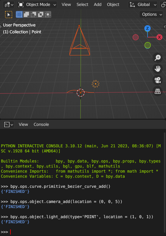
Operators include functions that perform the same task as the buttons and menu options in the Blender GUI. They only return the status of the operations, like in this image from the last section.
Tip
Camera added this way will not automatically become the active camera.
In the Python Console area, pressing Tab after typing the name of the function will give you a short documentation.
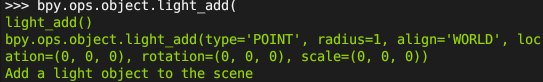
Apart from mesh objects, you can add curves, cameras, lights, etc., check the tooltips in the Add menu for the respective functions.
bpy.ops.curve.primitive_bezier_curve_add()
bpy.ops.object.camera_add(location = (0, 0, 5))
bpy.ops.object.light_add(type='POINT', location = (1, 0, 1))
You may want to delete everything before running the main part of the script, the following code can help:
Tip
This is good enough for the starting scene, but when applied to a complex scene it may not clean up everything.
bpy.ops.object.select_all(action="SELECT")
bpy.ops.object.delete()
bpy.ops.outliner.orphans_purge()
The first line selects everything in the scene (same as pressing A), the second deletes selected objects, and the last remove unused data from the file.
To Render a scene, run the following:
bpy.ops.render.render(write_still=True)
The write_still=True option saves the rendered image to the Output Path.
For complex setups, it might be easier to make it in Blender GUI and load the .blend file in Python script.
bpy.ops.wm.open_mainfile(filepath="PATH_TO_BLEND_FILE")
There are a lot more operators that can add modifiers, make keyframes, etc., but generally speaking, if you can achieve the same goal using both bpy.ops and bpy.data module, you should do it with bpy.data. Following that principle, we skip those operators in this section.
Data Access(bpy.data)#
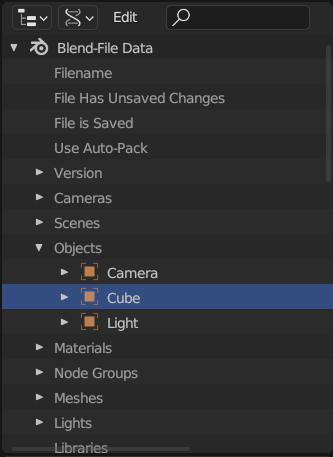
The Data Access is the most important module in the API, it allows you to access/create/modify data in the current file. An easy way to check the internal data structure is to switch the Display mode of an Outliner area to Data API.
For example, you can access the Cube object
bpy.data.objects["Cube"]
assign it to a variable
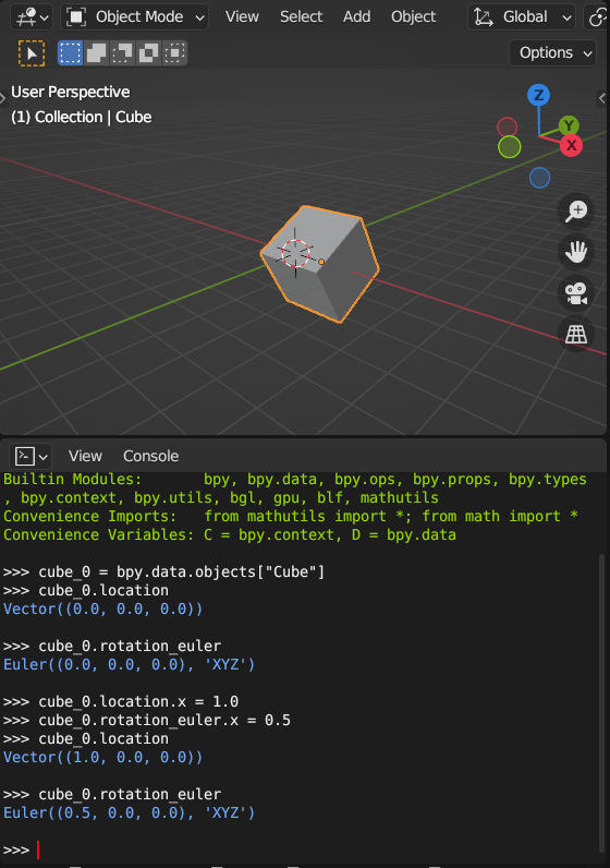
cube_0 = bpy.data.objects["Cube"]
and get/set its properties (location in this example)
Tip
Rotation angle is in radian, you can use math.radians() to turn degrees into radians.
cube_0.location
cube_0.rotation_euler
cube_0.location.x = 1.0
cube_0.rotation_euler.x = 0.5
You can add an object directly into the data. First, create a data-block for the object
cam_db = bpy.data.cameras.new("new_cam")
then use the data-block to construct a new object
cam_0 = bpy.data.objects.new("camera_0", cam_db)
and nothing happens in the viewport. But if you check the Data API, you will find both of them are there. To make it show up in the current scene, you need to link the object to a collection in the scene.
bpy.data.collections['Collection'].objects.link(cam_0)
Now it should be visible in the viewport.
Tip
This camera will not automatically become the active one.
Adding a collection to a scene is similar. Make a new collection in the data
ico_coll = bpy.data.collections.new("ico_collection")
then link the collection to the scene
bpy.data.scenes['Scene'].collection.children.link(ico_coll)
You can also loop through the objects in a collection
for obj in bpy.data.collections['ico_collection'].objects:
    obj.location.x += 1
Making a mesh object in bpy.data takes a bit more work than creating other objects. To make a mesh datablock, you need to define vertices, edges, and faces. Let’s look at this example:
verts = [
    (-1.0, -1.0, -1.0),
    (-1.0, 1.0, -1.0),
    (1.0, 1.0, -1.0),
    (1.0, -1.0, -1.0),
    (-1.0, -1.0, 1.0),
    (-1.0, 1.0, 1.0),
    (1.0, 1.0, 1.0),
    (1.0, -1.0, 1.0),
    ]

edges = [
    (0, 2),
]

faces = [
    (0, 1, 2, 3),
    (4, 5, 1, 0),
    (7, 6, 5, 4),
    (7, 4, 0, 3),
    (6, 7, 3, 2),
    (5, 6, 2, 1),
]
Tip
Turning on
indiceshelps visualizing the process.The order of the indices decides the how the face is constructed, and its normal follows the right-hand rule.
Vertices are naturally dictated by their coordinates, and faces are defined by the indices of vertices. The order of the indices is important for the faces, and the normal is determined by the right-hand rule. The edges are automatically generated where faces are defined, only additional edges are necessary. With these three lists ready, you can make the data-block
cube_mesh = bpy.data.meshes.new("cube_data")
cube_mesh.from_pydata(verts, edges, faces)
then create the mesh object and link it to the collection
cube_obj = bpy.data.objects.new("Cube_1", cube_mesh)
bpy.data.collections['Collection'].objects.link(cube_obj)
Tip
The added edge is not part of any faces.
You can add a modifier to an object in the data directly
cube_0.modifiers.new(name = "mod1", type = "SUBSURF")
And you can tweak it too
cube_0.modifiers['mod1'].levels = 3
cube_0.modifiers['mod1'].render_levels = 5
Adding a constraint is similar but it does not require a name.
cube_0.constraints.new(type = "LIMIT_LOCATION")
cube_0.constraints['Limit Location'].use_max_x = True
cube_0.constraints['Limit Location'].max_x = 1.0
cube_0.constraints['Limit Location'].use_transform_limit = True
To add keyframes, you need to specify the data path and frame
Tip
Data path:
Location: “location”
Rotation: “rotation_euler”
Scale: “scale”
cube_0.location = (2.0, 0.0, 0.0)
cube_0.keyframe_insert(data_path = "location", frame = 1)
cube_0.location = (-2.0, 0.0, 0.0)
cube_0.keyframe_insert(data_path = "location", frame = 250)
You can also delete keyframes
cube_0.keyframe_delete(data_path = "location", frame = 1)
cube_0.keyframe_delete(data_path = "location", frame = 250)
To add material to an object, first we need to create one in the data
mat = bpy.data.materials.new("new_mat")
then append it to the object
Tip
This creates a new material slot for the object.
cube_0.data.materials.append(mat)
Change the base color to see the effect
Tip
The diffuse color uses RGBA format.
mat.diffuse_color = (255.0, 0.0, 0.0, 1.0)
Unlike adding new material in the Material Properties, this material does not have a principled BSDF shader and does not use shader nodes. To make it consistent with what we did in the previous chapters, turn on Use Nodes.
Tip
More details in the coming Node Scripting section.
mat.use_nodes = True
You can change various scene properties with bpy.data. For example, you can change the end frame and frame rate
Tip
The index is 0 for the default scene, you can also use its name “Scene”.
bpy.data.scenes[index].frame_end = 120
bpy.data.scenes[index].render.fps = 30
You can also set the active camera
Tip
This set the camera object named “Camera” as active.
bpy.data.scenes[index].camera = bpy.data.objects['Camera']
and the Output Path, Render Engine, etc.
bpy.data.scenes[index].render.filepath = "YOUR_PATH"
bpy.data.scenes[index].render.engine = "CYCLES"
bpy.data.scenes[index].cycles.device = "GPU"
Drivers can be added through data access too. For example, if the cube has a Bevel modifier, you can add a driver to its Amount property like this
Tip
Check on which level you are adding the driver, for example, this does not work
cube_0.driver_add("modifiers['Bevel'].width")
cube_0.modifiers['Bevel'].driver_add("width")
For paths with indices such as location, rotation and scale, you can specify the index as the second argument
cube_0.driver_add("location", 0)
To make the driver work, first you need to add variables
loc_driver = cube_0.driver_add("location", 0)
var_0 = loc_driver.driver.variables.new()
var_0.name = "c_frame"
var_0.targets[0].id_type = "SCENE"
var_0.targets[0].id = C.scene
var_0.targets[0].data_path = "frame_current"
then use it to construct the expression
loc_driver.driver.expression = var_0.name + "/100"
Context Access(bpy.context)#
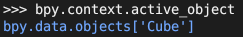
The Context Access module gives you easy access to the elements in the area currently being used. For example, when the cube is the active object (e.g. just added to the scene), instead of
cube_0 = bpy.data.objects["Cube"]
you can do
cube_0 = bpy.context.active_object
because it points to the same object in the data.
Similarly, to get the current scene, you can use
bpy.context.scene
which is the same as
bpy.data.scenes[index]
and we also have bpy.context.collection for the collection, bpy.context.engine for the render engine, etc.